Getting Started with EntropyScaling.jl
Installation
The package can be installed by:
Pkg> add EntropyScalingPackage mode can reached by typing ] in REPL. Then, the module can be loaded by
using EntropyScalingEOS Calculations
The calculation of transport properties through entropy scaling is mostly based on fundamental EOS (defined in the Helmholtz energy $a$) as they allow the consistent calculation of all required thermodynamic properties, in particular the configurational entropy $s_{\rm conf}$. The EOS calculations are not part of this package. Clapeyron.jl is used as thermodynamic backend for the EOS calculations providing a large number of different thermodynamic models.
using EntropyScaling, Clapeyron

eos_model = PCSAFT("n-butane")
model = ESFramework(eos_model, Dict(Viscosity() => [[0.;-14.165;13.97;-2.382;0.501;;]]))
η = viscosity(model, 37.21e6, 323.)
Units
EntropyScaling.jl can be used in combination with Unitful.jl. This enables both to obtain unitful properties directly from the models and to use data with associated units for fitting models.
- Unitful calculation of transport properties. This adds the methods:
viscosity(model, p::Pressure, T::Temperature, z=[1.]; phase=:unknown, output=default)viscosity(model, ϱ::Density, T::Temperature, z=[1.]; output=default)
::Propertyis meta code for unitful values, e.g.300u"K"forT::Temperature. The density can either be mass or molar density. Theoutputkeyword defines the unit of the calculated transport property (see here for the default values). - Defining data for fitting entropy scaling models using units. This supports constructing
TransportPropertyDatausing units, e.g.TransportPropertyData(T::Vector{Temperature}, p::Vector{Pressure}, η::Vector{Viscosity}). The property-specific constructors (ViscosityData, ...) also support units.
In the following, both cases are demonstrated:
using EntropyScaling, Unitful, Clapeyron, CoolProp

# Calculate unitful transport properties
model_ref = RefpropRES("methane")
thermal_conductivity(model_ref, 1u"atm", 80u"°F")
# 0.019529950158013242 W K^-1 m^-1

# Assign units to data for fitting
(_T_exp,_ϱ_exp,_η_exp) = EntropyScaling.load_sample_data();     # Load sample data
T_exp = _T_exp .* 1u"K"
ϱ_exp = _ϱ_exp .* 1u"mol/m^3"
η_exp = _η_exp .* 1u"Pa*s"

data = TransportPropertyData(T_exp, ϱ_exp, η_exp)

eos_model = PCSAFT("butane")
model = ESFramework(eos_model, [data])                          # Fit model parameters

η = viscosity(model, 1u"bar", 26.85u"°C", phase=:liquid, output = u"cP")
# 0.16058971694885213 cP
Visualization
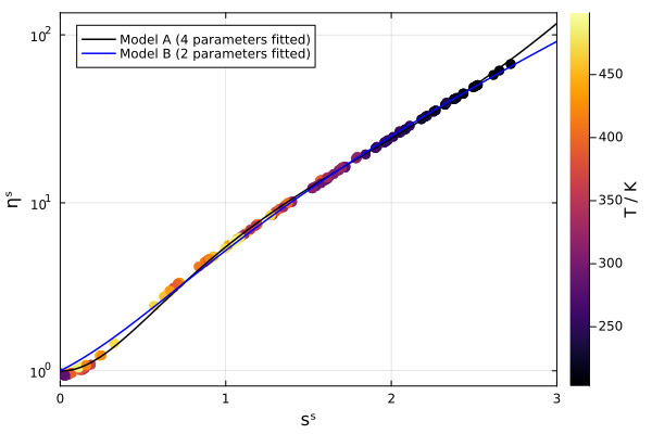
Plotting functionality is available through extensions to Makie.jl and Plots.jl. In particular, "entropy scaling" plots, i.e. the scaled transport property $Y^s$ as function of the scaled entropy $s^s$, can easily be created as described below.
EntropyScaling.plot_scaling — Function
plot_scaling(model::AbstractEntropyScalingModel, dat::TransportPropertyData; kwargs...)
plot_scaling!(model::AbstractEntropyScalingModel, dat::TransportPropertyData; kwargs...)
plot_scaling!(axis, model::AbstractEntropyScalingModel, dat::TransportPropertyData; kwargs...)
Plots the scaled transport property as a function of the entropy-scaling variable (e.g. the reduced entropy). The entropy scaling model as well as the scaled transport property data are shown.
Arguments
model: An entropy scaling model containing transport property parametersdata: Transport property data to plot (ornothing)axis: An existing axis to add the plot
Keyword Arguments
slims: Sets the range for the entropy scaling variable (used for the model calculation)prop: Sets the transport property (only required ifdat == nothing)cprop: Controls the property used for coloring (e.g.:T,:p, orϱ)marker: Shape of markers for data points (default::circle)markersize: Size of markers for data points (default: depends on plot package)markercolor: Color of markers when not using property-based coloring (default::blue)colormap: Colormap to use for coloring points (default::viridis)colorrange: Range of values for the colorbar (default: extrema of the property used for coloring)linecolor: Color of the model line (default::black)linewidth: Width of the model line (default:2)linestyle: Style of the model line (default::solid)label: Label for legend entries (default:nothing)
Supported Plot Packages
- Makie.jl: Import a specific backend, e.g.
using CairoMakieorusing GLMakie. - Plots.jl: Import with
using Plots.
Example
In the following example, entropy scaling models are fitted to quasi-experimental data (from CoolProp) and compared.
using EntropyScaling, Clapeyron, CoolProp
using GLMakie

# Create synthetic data
sub = "propane"
T, p = rand(200.:500.,200), 10.0.^(rand(200).*4 .+ 4)
η = [PropsSI("V","T",T[i],"P",p[i],sub) for i in 1:200]

# Create data and model
ηdat = ViscosityData(T,p,nothing,η)
model_A = ESFramework(PCSAFT(sub), [ηdat])
model_B = ESFramework(PCSAFT(sub), [ηdat]; opts=FitOptions(what_fit=Dict(Viscosity() => Bool[0,1,0,1,0])))

# Plot
fig = plot_scaling(model_A, ηdat; cprop=:T, linewidth=3, linecolor=:blue, label="model A (4 parameters)")
plot_scaling!(model_B, nothing; slims=(0,3), prop=Viscosity(), linestyle=:dash, label="model B (2 parameters)")
axislegend(position=:lt, framevisible=false)
ax2 = Axis(fig[2,1])
plot_scaling!(ax2, model_A, ηdat; marker=:star5, markercolor=:red, label="model A again")
axislegend(position=:lt, framevisible=false)
ax2.yscale = identity
fig